Visualizing Language Loss in Taiwan
Create an “Age-Sex Pyramid of Language” with ggplot2
Taiwan Language Survey is a small project I worked on during May to June in 2018. The idea was to create a survey that continuously collects data and a web page that visualizes the collected data. The web page is updated weekly using Travis-CI.
The main purpose of this survey is to raise public awareness of language loss in Taiwan. Hence, the survey is designed to collect data that can provide valuable information about language loss, for example, some questions were asked to gain insight about the change of linguistic competence acoss generations in a family (i.e. across the subject’s parents, the subject, and the subject’s children). In addition to changes within family, information about the age of the subjects is also colleceted, meaning that we can see how linguistic competence changes among diffrent age groups of subjects in a community, i.e. is a language becoming more dominant or entering the dying process?
Visualization is a powerful tool to capture how linguistic competences of different langauges are changing. But creating visualizations necessitates creativity – how can language loss be visualized? Below, I illustrate one of the methods I created for visualizing language loss – a visaulization inspired by the age-sex pyramid.
Age-Sex Pyramid of Language
The age-sex pyramid is used to visualize the population structure of a community. The vertical axis indicates the age and each horizontal bar represents an age group. The horizontal axis indicates the population size of male or female of a particular age group.
The age-sex pyramid is a great tool to visualize the population structure since the ‘shape’ of the pyramid gives readers a lot information. For example, an ‘expansive pyramid’ has longer bars at the bottom of the pyramid, which indicates the population is young and growing. A ‘stationary pyramid’ looks like a rectangular bar, indicating the population sizes of different age groups are about the same. A ‘constructive’ pyramid indicates a shrinking population, which is narrowed at the bottom.
Similarly, a modified version of the age-sex pyramid, which I’ll call the ‘age-sex pyramid of language’, can be used to visualize the population structure of a language and predicts the language’s vitality. Instead of visualizing population size, the age-sex pyramid of language visualizes the average fluency of a language on the horizontal axis.
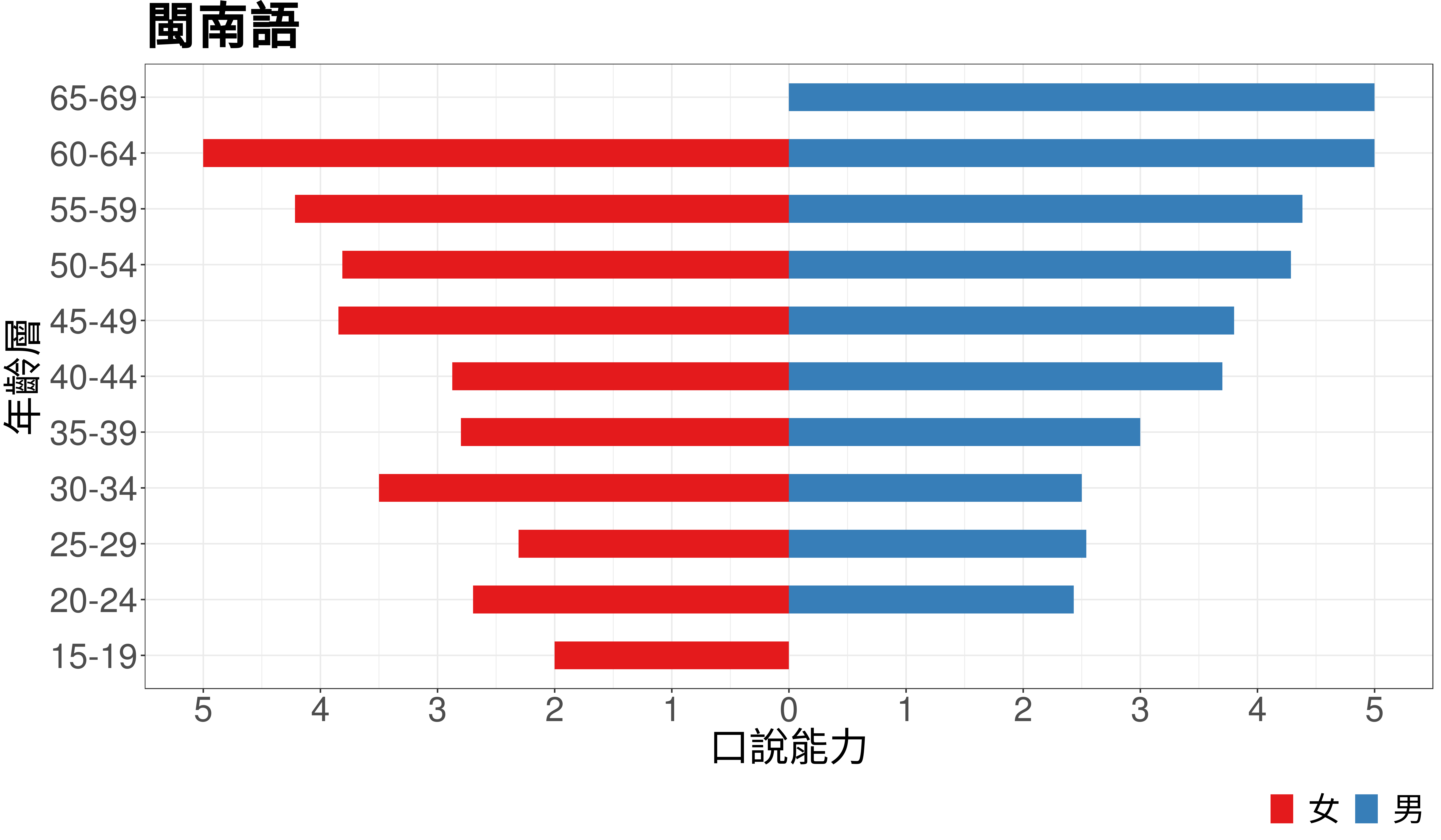
Figure 1: An age-sex pyramid of Taiwanese. The red bars on the left indicates females of different age groups and the blue bars on the right indicates males. The average fluency (values on the horizontal axis) is calculated from a six-point scale (0-5) on Taiwanese fluency.
As shown in Figure 1, the shape of the age-sex pyramid of Taiwanese in Taiwan1 is an ‘inverted triangle’, which is almost never seen in the conventional population pyramid. However, this inverted triangular shape is expected to appear quite often, since it indicates an ongoing language loss in a community.
| Vitality of Language | Shape of Pyramid |
|---|---|
| Shrinking and Dying | Inverted Triangle |
| Growing | Triangle |
| Stable | Rectangular Bar |
Drawing Age-Sex Pyramid with ggplot2
As complex as it might seem, an age-sex pyramid created with ggplot2 is actually a (modified) bar chart. I learned this on stackoverflow, and the trick is
- Use
ifelseto flip the value (here, population size) according to the gender of the age group - Use
geom_bar(stat = "identity")to let the heights of the bars represent values in the data frame, i.e. the value given toy - Use
coord_flip()to make the bars horizontal
set.seed(1)
df0 <- tibble::tibble(
  Age = rep(c('10-19', '20-29', '30-39'), 2),
  Gender = rep(c('Female', 'Male'), each = 3),
  PopSize = sample(0:100, size = 6, replace = T)
  )
df0| Age | Gender | PopSize |
|---|---|---|
| 10-19 | Female | 26 |
| 20-29 | Female | 37 |
| 30-39 | Female | 57 |
| 10-19 | Male | 91 |
| 20-29 | Male | 20 |
| 30-39 | Male | 90 |
library(ggplot2)
pl <- ggplot(df0, aes(x = Age,
                      y = ifelse(Gender == 'Male', PopSize, -PopSize),
                      fill = Gender)) +
  geom_bar(stat = 'identity') +
  coord_flip()
pl
To center the plot (i.e. to make the point where population size is zero at the center of the plot), we have to scale the axis of ‘population size’ (y) with scale_y_continuous:
pl + scale_y_continuous(limits = c(-100, 100),
                        breaks = seq(-100, 100, 25),
                        labels = abs) +
  labs(y = 'Population Size')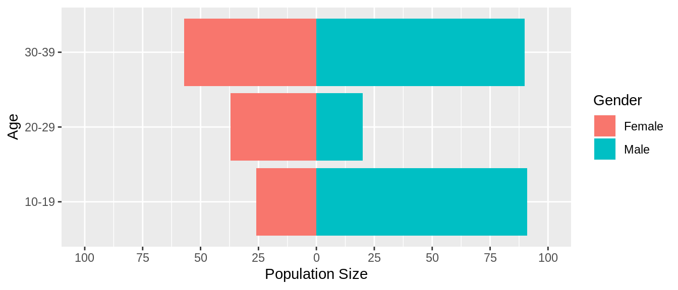
where abs in labels is the function abs(). By default, ggplot2 pass the value given in breaks to the the function specified in labels.
Visualizing Language Loss
To create an age-sex pyramid of language, the data structure needed is exactly the same as the one above, except the variable, PopSize, is replaced by ‘average fluency’ of a language. But since most people in Taiwan can speak more than one language (e.g. Mandarin-Taiwanese, Mandarin-Taiwanese-Hakka, Mandarin-English, etc.), the real data from the survey is a bit more complex Basically, the data structure needed to draw an age-sex pyramid of language looks like:
| Gender | Ethnicity | Age Group | Avg. Fluency |
|---|---|---|---|
| female | Mandarin | 20-24 | 4.53 |
| male | Taiwanese | 20-24 | 2.78 |
| … | … | … | … |
| female | Hakka | 25-29 | 2.23 |
| male | Taiwanese | 35-39 | 3.57 |
Preparation of Data
The raw data of Taiwan Language Survey can be retrieved here. The survey and raw data is in traditional Chinese. I’ll skip the step of cleaning raw data (e.g., turn variable names to English) and used the cleaned data survey.rds instead.
temp <- tempfile()
download.file('https://raw.githubusercontent.com/twLangSurvey/twLangSurvey.github.io/master/data/survey.rds', destfile = temp)
data <- readr::read_rds(temp)
head(data, 3)| date | curr_resid | curr_resid_since | settle_5yy | home_town | gender | age | kid_num | edu_level | work | income | work_hr | tribe | Mand_listen | Mand_speak | Tw_listen | Tw_speak | Hak_listen | Hak_speak | Ind_listen | Ind_speak | SEA_listen | SEA_speak | Eng_listen | Eng_speak | first_lang | when_Mand | when_Tw | when_Hak | when_Ind | when_SEA | when_Eng | m_guard_identity | f_guard_identity | dad_Mand_speak | dad_Tw_speak | dad_Hak_speak | dad_Eng_speak | dad_Ind_speak | dad_SEA_speak | mom_Mand_speak | mom_Tw_speak | mom_Hak_speak | mom_Eng_speak | mom_Ind_speak | mom_SEA_speak | dad_mom_Mand_fq | dad_mom_Tw_fq | dad_mom_Hak_fq | dad_mom_Ind_fq | dad_mom_SEA_fq | dad_mom_Other_fq | me_dad_Mand_fq | me_dad_Tw_fq | me_dad_Hak_fq | me_dad_Ind_fq | me_dad_SEA_fq | me_dad_Other_fq | me_mom_Mand_fq | me_mom_Tw_fq | me_mom_Hak_fq | me_mom_Ind_fq | me_mom_SEA_fq | me_mom_Other_fq |
|---|---|---|---|---|---|---|---|---|---|---|---|---|---|---|---|---|---|---|---|---|---|---|---|---|---|---|---|---|---|---|---|---|---|---|---|---|---|---|---|---|---|---|---|---|---|---|---|---|---|---|---|---|---|---|---|---|---|---|---|---|---|---|---|
| 2018-06-12 | 106 | 1996 | 是 | 428 | 女 | 56 | 2 | 大學 | 金融業 | 10萬以上 | 45 - 50 小時 | 不具原住民身份 | 5 | 4 | 3 | 2 | 0 | 0 | 0 | 0 | 0 | 0 | 2 | 1 | 華語 | 7歲前 | 7歲前 | 未學會 | 未學會 | 未學會 | 12-15歲 | 父親 | 母親 | 3 | 0 | 0 | 0 | 0 | 0 | 3 | 4 | 0 | 0 | 0 | 0 | 幾乎全用 | 幾乎不用 | 幾乎不用 | 幾乎不用 | 幾乎不用 | 幾乎不用 | 幾乎全用 | 幾乎不用 | 幾乎不用 | 幾乎不用 | 幾乎不用 | 幾乎不用 | 約一半 | 多數使用 | 幾乎不用 | 幾乎不用 | 幾乎不用 | 幾乎不用 |
| 2018-06-13 | 204 | 2004 | 是 | 204 | 女 | 57 | 1 | 碩士 | 製造業 | 10萬以上 | 50 - 55 小時 | 不具原住民身份 | 5 | 5 | 5 | 5 | 0 | 0 | 0 | 0 | 0 | 0 | 4 | 4 | 華語 | 7歲前 | 7歲前 | 未學會 | 未學會 | 未學會 | 12-15歲 | 父親 | 母親 | 5 | 5 | 0 | 1 | 0 | 0 | 1 | 5 | 0 | 0 | 0 | 0 | 幾乎不用 | 多數使用 | 幾乎不用 | 幾乎不用 | 幾乎不用 | 幾乎不用 | 幾乎不用 | 多數使用 | 幾乎不用 | 幾乎不用 | 幾乎不用 | 幾乎不用 | 幾乎不用 | 多數使用 | 幾乎不用 | 幾乎不用 | 幾乎不用 | 幾乎不用 |
| 2018-06-13 | 103 | 2013 | 是 | 100 | 男 | 37 | 2 | 大學 | 金融業 | 55,000 - 60,000 | 25 - 30 小時 | 不具原住民身份 | 5 | 5 | 2 | 1 | 0 | 0 | 0 | 0 | 0 | 0 | 3 | 2 | 華語 | 7歲前 | 未學會 | 未學會 | 未學會 | 未學會 | 7-12歲 | 父親 | 母親 | 5 | 5 | 5 | 1 | 0 | 0 | 5 | 3 | 0 | 4 | 0 | 0 | 幾乎全用 | 少數使用 | 幾乎不用 | 幾乎不用 | 幾乎不用 | 幾乎不用 | 多數使用 | 少數使用 | 幾乎不用 | 幾乎不用 | 幾乎不用 | 幾乎不用 | 幾乎全用 | 幾乎不用 | 幾乎不用 | 幾乎不用 | 幾乎不用 | 幾乎不用 |
The survey data, data, contains 22 variables and 267 observations (subjects). I only need these variables below to create the plot I want:
gender: The gender of the subjectage: The age of the subjectm_guard_identity: Male guardian of the subject, should be ‘father’ in most casesf_guard_identity: Female guardian of the subject, should be ‘mother’ in most cases<lang>_speak: The subject’s fluency of a language.<lang>is one of ‘Mand’ (Mandarin), ‘Tw’ (Taiwanese), ‘Hak’ (Hakka), ‘Ind’ (languages of the indigenous peoples, aka Formosan languages, belong to Austronesian languages), ‘SEA’ (languages from South Easth Asia), and ‘Eng’ (English)dad_<lang>_speak: The subject’s male guardian’s fluency of a language.<lang>is same as above.mom_<lang>_speak: The subject’s female guardian’s fluency of a language.<lang>is same as above.
library(dplyr)
lang <- c('Mand', 'Tw', 'Hak', 'Ind', 'SEA', 'Eng')
cols <- c('gender', 'age', 'm_guard_identity', 'f_guard_identity',
          paste0(lang, '_speak'),
          paste0('dad_', lang, '_speak'),
          paste0('mom_', lang, '_speak')
          )
data <- data[, cols] %>%
    filter(gender == '男' | gender == '女')
Since some content of the survey data is in Chinese, the code below is used to translate it to English:
ch2eng <- function(x) {
  if (x == '男') return('Male')
  if (x == '女') return('Female')
  if (x == '母親') return('Mother')
  if (x == '父親') return('Father')
  if (x == '無') return('None')
  if (x == '(外)祖父') return('Grandpa')
  if (x == '(外)祖母') return('Grandma')
  if (x %in% c('阿姨', '嬸嬸', '舅媽', '姑姑', '伯母')) return('Aunt')
  if (x %in% c('叔叔', '伯伯', '舅舅', '姑丈', '姨丈')) return('Uncle')
  message('No translation found for `', x, '`', '\n')
  return(x)
}

ch2eng_vec <- function(vec) {
  new_vec <- vector(typeof(vec), length(vec))
  for (i in seq_along(vec)) {
    new_vec[[i]] <- ch2eng(vec[[i]])
  }
  return(new_vec)
}

data <- data %>%
  mutate(gender = ch2eng_vec(gender),
         m_guard_identity = ch2eng_vec(m_guard_identity),
         f_guard_identity = ch2eng_vec(f_guard_identity))
head(data)| gender | age | m_guard_identity | f_guard_identity | Mand_speak | Tw_speak | Hak_speak | Ind_speak | SEA_speak | Eng_speak | dad_Mand_speak | dad_Tw_speak | dad_Hak_speak | dad_Ind_speak | dad_SEA_speak | dad_Eng_speak | mom_Mand_speak | mom_Tw_speak | mom_Hak_speak | mom_Ind_speak | mom_SEA_speak | mom_Eng_speak |
|---|---|---|---|---|---|---|---|---|---|---|---|---|---|---|---|---|---|---|---|---|---|
| Female | 56 | Father | Mother | 4 | 2 | 0 | 0 | 0 | 1 | 3 | 0 | 0 | 0 | 0 | 0 | 3 | 4 | 0 | 0 | 0 | 0 |
| Female | 57 | Father | Mother | 5 | 5 | 0 | 0 | 0 | 4 | 5 | 5 | 0 | 0 | 0 | 1 | 1 | 5 | 0 | 0 | 0 | 0 |
| Male | 37 | Father | Mother | 5 | 1 | 0 | 0 | 0 | 2 | 5 | 5 | 5 | 0 | 0 | 1 | 5 | 3 | 0 | 0 | 0 | 4 |
| Female | 44 | Father | Mother | 5 | 4 | 0 | 0 | 0 | 4 | 5 | 5 | 0 | 0 | 0 | 0 | 5 | 5 | 0 | 0 | 0 | 0 |
| Male | 62 | None | None | 5 | 5 | 0 | 0 | 0 | 1 | 5 | 0 | 4 | 0 | 0 | 0 | 5 | 5 | 0 | 0 | 0 | 0 |
| Female | 56 | Father | Mother | 5 | 5 | 0 | 0 | 0 | 1 | 5 | 5 | 0 | 0 | 0 | 0 | 5 | 5 | 0 | 0 | 0 | 0 |
Defining Ethnicity
You might notice that there is no variable in the data which explicitly indicates the ethnicity of the subject. To serve the purpose of this survey – visualizing the vitality of languages in a community, ethnicity is defined solely by the linguistics competence of a subject’s guardians.
To give a specific example, let subject A has a mother who can speak2 Mandarin and Taiwanese and a father who speaks Mandarin and Hakka, then subject A is categorized as a Mandarin, a Taiwanese, and a Hakka simultaneously.
The function filter_ethnic() is used to filter out subjects with specified ‘ethnicity’. This function is useful for drawing age-sex pyramid for each of the six languages.
filter_ethnic <- function(df, lang, lev = 3) {
    sp_lang <- vector("character", 3)
    sp_lang[1] <- paste0("dad_", lang, "_speak")
    sp_lang[2] <- paste0("mom_", lang, "_speak")
    sp_lang[3] <- paste0(lang, "_speak")

    df2 <- df %>%
      filter(m_guard_identity != 'None' | f_guard_identity != 'None') %>%
      filter(.data[[sp_lang[1]]] >= lev | .data[[sp_lang[2]]] >= lev) %>%
      select(age, gender, sp_lang)
    return(df2)
}
Assinging Age Group to Subjects
Remember that the data structure needed for plotting age-sex pyramids requires age group to be the basic unit. data now consisits of single subjects, and we need information to group subjects together according to their ages. mutate_age_group() creates a new variable age_group by the subject’s age.
mutate_age_group <- function(df, range = 5){
    df$age_group <- as.character(
      cut(df$age, right = F, breaks = seq(10, 95, by = range))
    )
    return(df)
}
cut() takes a numeric vector as its first input, and codes the values of the vector into new values according to the interval they fall into. In mutate_age_group(), cut() codes the input vectors according to the intervals specified in the argument breaks.
Now we can use these functions to add more information to the data frame. The idea is to first create a separated data frame for each ethnicity3 (by filter_ethnic()), then attact new variables to the data frame that indicate a subject’s ethnicity (ethn_group) and age group (age_group).
lang <- c('Mand', 'Tw', 'Hak', 'Ind', 'SEA', 'Eng')
lev <- c(3, 3, 3, 3, 3, 0)
ethn_list_df <- vector("list", length(lang))

for (i in seq_along(lang)){
  ethn_list_df[[i]] <- filter_ethnic(data,
                                     lang = lang[i],
                                     lev = lev[i]) %>%
    mutate(ethn_group = lang[i]) %>%
    mutate_age_group() %>%
    select(age, gender, age_group, ethn_group,
           paste0(lang[i], "_speak")) %>%
    rename(lang_fluency = paste0(lang[i], "_speak"))
}
Then we can recombine these data frames back to a single one, and this new data frame now has information about a subject’s ethinicity and age group he/she belongs to. (Note that the new data frame is expended since one subject can have several ethnicity, i.e. one subject can appear in different rows of the data frame with different ethnicity.)
bind_rows(ethn_list_df) %>% head()| age | gender | age_group | ethn_group | lang_fluency |
|---|---|---|---|---|
| 56 | Female | [55,60) | Mand | 4 |
| 57 | Female | [55,60) | Mand | 5 |
| 37 | Male | [35,40) | Mand | 5 |
| 44 | Female | [40,45) | Mand | 5 |
| 56 | Female | [55,60) | Mand | 5 |
| 53 | Male | [50,55) | Mand | 5 |
Data for Plotting
Finally, we are ready to group the subjects together according to his/her gender, ethnicity, and age_group. After grouping, we can use dplyr::summarise() to calculate each group’s fluency of the language, which will be used as the variable on the horizontal axis of the age-sex pyramid.
pl_data <- bind_rows(ethn_list_df) %>%
  group_by(gender, ethn_group, age_group) %>%
  summarise(mean(lang_fluency)) %>%
  rename(avg_fluency = `mean(lang_fluency)`)

head(pl_data)| gender | ethn_group | age_group | avg_fluency |
|---|---|---|---|
| Female | Eng | [15,20) | 1.750 |
| Female | Eng | [20,25) | 2.950 |
| Female | Eng | [25,30) | 2.600 |
| Female | Eng | [30,35) | 3.000 |
| Female | Eng | [35,40) | 1.750 |
| Female | Eng | [40,45) | 2.125 |
Plotting Function
We are going to draw 6 age-sex pyramids, one for each languages. So instead of writing ggplot() six times, I wrote a plotting function:
library(ggplot2)
pl_pyramid <- function(data, title = NULL) {
  ggplot(data,
         aes(x = age_group,
             y = ifelse(gender == 'Male', avg_fluency, -avg_fluency),
             fill = gender)) +
  geom_bar(stat = "identity", width = 0.7) +
  scale_y_continuous(limits = c(-5, 5),
                     breaks = seq(-5, 5, 1),
                     labels = abs(seq(-5, 5, 1))) +
  coord_flip() +
  scale_fill_manual(values = c("#E41A1C", "#377EB8"),
                    breaks = c("Female", "Male")) +
  labs(x = "Age", y = "Fluency", fill = "", title = title)
}
Now we can start plotting. Let’s try Mand (Mandarin) and Hak (Hakka) first. We can use dplyr::filter() to filter out people speaking these languages:
tweak <-  theme_bw() +
  theme(axis.text = element_text(size = 15),
        legend.justification = "right",
        legend.position = "bottom",
        legend.box = "vertical")

pl_data %>%
  filter(ethn_group == 'Mand') %>%
  pl_pyramid(title = 'Mandarin') + tweak

pl_data %>%
  filter(ethn_group == 'Ind') %>%
  pl_pyramid(title = 'Formosan Languages') + tweak

Wait! It seems quite strange. The age-sex pyramid of ‘Formosan Languages’ doesn’t look like a pyramid at all! This is because there were very few subjects defined as ‘indigenous people’ in the survey. To make plots like this (with only one or two age groups) comparable to others (such as that in ‘Mandarin’), we need one more function to insert missing age groups to the data frame so that ggplot can draw empty bars for us.
First, we need to find out all age groups in the data:
age_groups <- unique(pl_data$age_group)
age_groups
[1] "[15,20)" "[20,25)" "[25,30)" "[30,35)" "[35,40)" "[40,45)" "[45,50)"
[8] "[50,55)" "[55,60)" "[60,65)" "[65,70)"Then we can write a function fill_empty_age_group(), which takes a data frame as its first argument and checks whether there are age groups missing in the data frame (using its second argument, age_group_all, as comparison). If the age group is missing, fill_empty_age_group() appends a new row, which has age_group set to the missing age group and avg_fluency set to 0 (create an empty bar), to the input data frame.
fill_empty_age_group <- function(df, age_group_all) {
  for (i in seq_along(age_group_all)) {
    if (!(age_group_all[i] %in% df$age_group)) {
      df <- rbind(df, list(gender = "Female",
                           ethn_group = "doesnt_matter",
                           age_group = age_group_all[i],
                           avg_fluency = 0))
    }
  }
  return(df)
}
Now we’re ready to explore language loss in Taiwan. multiplot() is used to put multiple plots together. The source code of multiplot() is copied directly from Winston Chang’s Cookbook for R.
tweak2 <-  theme_bw() +
  theme(legend.justification = "right",
        legend.position = "bottom",
        legend.box = "vertical")

py1 <- pl_data %>%
  filter(ethn_group == 'Mand') %>%
  fill_empty_age_group(age_groups) %>%
  pl_pyramid(title = 'Mandarin') + tweak2

py2 <- pl_data %>%
  filter(ethn_group == 'Tw') %>%
  fill_empty_age_group(age_groups) %>%
  pl_pyramid(title = 'Taiwanese') + tweak2

py3 <- pl_data %>%
  filter(ethn_group == 'Hak') %>%
  fill_empty_age_group(age_groups) %>%
  pl_pyramid(title = 'Hakka') + tweak2

py4 <- pl_data %>%
  filter(ethn_group == 'Ind') %>%
  fill_empty_age_group(age_groups) %>%
  pl_pyramid(title = 'Formosan Languages') + tweak2

py5 <- pl_data %>%
  filter(ethn_group == 'SEA') %>%
  fill_empty_age_group(age_groups) %>%
  pl_pyramid(title = 'Languages of South East Asia') + tweak2

py6 <- pl_data %>%
  filter(ethn_group == 'Eng') %>%
  fill_empty_age_group(age_groups) %>%
  pl_pyramid(title = 'English') + tweak2

multiplot(py1, py2, py3, py4, py5, py6, cols = 2)
Language Loss in Taiwan
As described in Age-Sex Pyramid of Language above, we can learn about a language’s vitality in Taiwan from the age-sex pyramids drawn above.
For Formosan and South East Asian languages, there are too few data, and we can’t learn much about these languages from the plots. For Mandarin, the shape of the pyramid is rectangular, indicating the linguistic competence of Mandarin is stable across people of all ages. This is expected as Mandarin, in Taiwan, is the most prevalent language, and most people use it as the primary language in workplace and home.
Pyramids of Taiwanese and Hakka have inverted trianglular shapes, indicating lower linguistic competence among yonger people. Indeed, it’s not uncommmon to see the fathers and mothers talk to their children in Mandarin but talk to their parents in Taiwanese. Taiwanese is the second prevalent language in Taiwan, but it is shrinking, particularly among young people. Hakka ranks third in prevalence. It faces similar situation to Taiwanese but the situation is even worse, since the usage of Hakka is mostly restricted to Hakka people whereas usage of Taiwanese is not restricted to particular groups of people (many indigenous and Hakka peoples speak fluent Taiwanese).
English has a special status in Taiwan. It is not a native tongue to people born and raised in Taiwan, but many people know at least a little English. This is because formal education and the (awareness of) globalization lead parents to place importance on English education of their children. This also gives the age-sex pyramid of English its appearance – a triangular shape with wider bottom than top. English is the only language that is growing in Taiwan and, arguably, the language with the strongest vitality. Table 1 summarizes the discussion above.
| Vitality of Language | Shape of Pyramid | Examples (Taiwan) |
|---|---|---|
| Shrinking and Dying | Inverted Triangle | Taiwanese, Hakka |
| Growing | Triangle | English |
| Stable | Rectangular Bar | Mandarin |
The samples are not representative though, and it might only reflect the situation in Taipei (see the geographical distribution of the samples below). But I think there are still reasons to believe that other locations in Taiwan have similar phenomena.
Defined by scoring 3 or above in a self-reported 6-point scale measuring the fluency of a language spoken by the subject’s parents.↩
For English, different from all other languages, the level used to determine ethnicity is
0, i.e. there is no filtering occuring, and all subjects are used. This is because, in Taiwan (and many other non-English speaking communities as well), English is not related to ethnicity and is strongly related to formal education and job requirements.↩

Last updated: 2019-04-03