Demystifying Item Response Theory (1/4)

Mysterious Item Response Theory

Item response theory is mysterious and intimidating to students. It is mysterious in the way it is presented in textbooks, at least in introductory ones. The text often starts with an ambitious conceptual introduction to IRT, which most students would be able to follow, but with some confusion. Curious students might bear with the confusion and expect it to resolve in the following text, only to find themselves disappointed. At the point where the underlying statistical model should be further elaborated, the text abruptly stops and tries to convince the readers to trust the results from black-box IRT software packages.

It isn’t that I have trust issues with black-box software, and I also agree that certain details of IRT model estimation should be hidden from the readers. The problem is that there’s a huge gap here, between where textbooks stopped explaining and where the confusing details of statistics should be hidden. Hence, students would be tricked into believing that they have a sufficient degree of understanding, but in reality, it’s just blind faith.

A sufficient degree of understanding should allow the student to deploy the learned skills to new situations. Therefore, a sufficient degree of understanding of IRT models should allow students to extend and apply the models to analyses of, for instance, differential item functioning (DIF) or differential rater functioning (DRF).

I’m arguing here that there is a basic granularity of understanding, somewhat similar to the concept of basic-level category, that when reached, allows a student to smoothly adapt the learned skills to a wide variety of situations, modifying and extending the skills on demand. And I believe that item response theory is too hard for a student to learn and reach this basic level of understanding, given its conventional presentation and historical development¹.

There is still hope however, thanks to the development of a very general set of statistical models known as the Generalized Linear Models (GLM). Item response models could be understood in terms of the GLM and its extensions (GLMM and non-linear form of the GLM/GLMM). To be too particular about the details, the results from IRT software packages and the GLMs/GLMMs would be very similar but not identical, since they utilize different estimation methods. The strengths of the GLM, however, lie in its conceptual simplicity and extensibility. Through GLM, IRT and other models such as the T-test, ANOVA, and linear regression, are all placed together into the same conceptual framework. Furthermore, software packages implementing GLMs are widely available. Users can thus experiment with them—simulate a set of data based on known parameters, construct the model and feed it the data, and see if the fitted model correctly recovers the parameters. This technique of learning statistics is probably the only effective way for students to understand a mysterious statistical model.

In this series of posts, I will walk you through the path of understanding item response theory, with the help of simulations and generalized linear models. No need to worry if you don’t know GLMs yet. We have another ally—R, in which we will be simulating artificial data and fitting statistical models along the way. Although it might seem intimidating at first, coding simulations and models in fact provide scaffolding for learning. When feeling unsure or confused, you can always resort to these simulation-based experiments to resolve the issues at hand. In this very first post, I will start by teaching you simulations.

Just Enough Theory to Get Started

Jargons aside, the concept behind item response theory is fairly simple. Consider the case where 80 testees are taking a 20-item English proficiency test. Under this situation, what are the factors that influence whether an item is correctly solved by a testee? Straightforward right? If an item is easy and if a testee is proficient in English, he/she would probably get the item correct. Here, two factors jointly influence the result:

1. how difficult (or easy) the item is
2. the English ability of the testee

We can express these variables and the relations between them in the graphs below. Let’s focus on the left one first. Here, $A$ represents the ability of the testee, $D$ represents the difficulty of the item, and $R$ represents the item response, or score on the item. A response for an item is coded as 1 ($R=1$) if it is solved correctly. Otherwise, it is coded as 0 ($R=0$). The arrows $A \rightarrow R$ and $D \rightarrow R$ indicate the direction of influence. The arrows enter $R$ since item difficulty and testee ability influence the score on the item (not the other way around). $A$ and $D$ are drawn as a circled node to indicate that they are unobserved (or latent, if you prefer a fancier term), whereas uncircled nodes represent directly observable variables (i.e., stuff that gets recorded during data collection). This graphical representation of the variables and their relationships is known as a Directed Acyclic Graph (DAG).

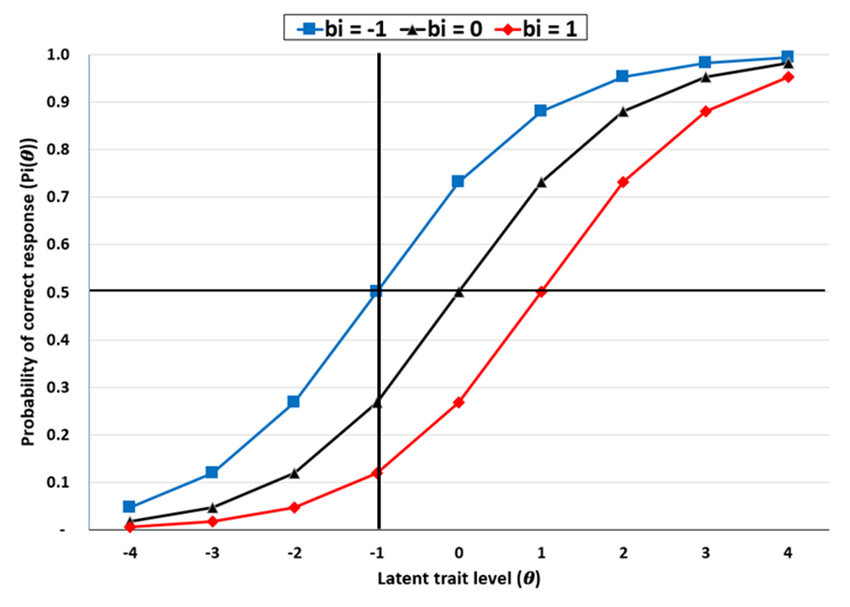
The DAGs laid out here represent the concept behind the simplest kind of item response models, known as the 1-parameter logistic (1PL) model (or the Rasch Model). In more formal terms, this model posits that the probability of correctly answering an item is determined by the difference between testee ability and item difficulty. So a more precise DAG representation for this model would be the one shown on the right above. Here, $P$ is the probability of correctly answering the item, which cannot be directly observed. However, $P$ directly influences the item score $R$, hence the arrow $P \rightarrow R$.

Believe it or not, the things we have learned so far could get us started. So let’s simulate some data, based on what we’ve learned about item response theory!

Simulating Item Responses

Consider the scenario where 3 students (Rob, Tom, and Joe) took a math test with 2 items (A and B). Since we play gods during simulations, we know the math ability of the students and the difficulty of the items. These ability/difficulty levels can range from positive to negative numbers, unbounded. Larger numbers indicate higher levels of difficulty/ability. In addition, the levels of difficulty and ability sit on a common scale and hence could be directly compared. Also, each student responds to every item, so we get responses from all 6 (3x2) combinations of students and items. Let’s code this in R below. The function expand.grid() would pair up the 6 combinations for us.

1D = c( A=0.4, B=0.1 )  # Difficulty of item
2A = c( R=0.5, T=0.1, J=-0.4 )  # Ability of student (R:Rob, T:Tom, J:Joe)
3
4dat = expand.grid( 
5   I = c( "A", "B" ),      # Item index
6   T = c( "R", "T", "J" )  # Testee index
7)
8dat

# A tibble: 6 x 2
  I     T    
  <fct> <fct>
1 A     R    
2 B     R    
3 A     T    
4 B     T    
5 A     J    
6 B     J    

After having all possible combinations of the students and the items, we could collect the values of student ability and item difficulty into the data frame.

1dat$A = A[ dat$T ]  # map ability to df by testee index T
2dat$D = D[ dat$I ]  # map difficulty to df by item index I
3dat

# A tibble: 6 x 4
  I     T         A     D
  <fct> <fct> <dbl> <dbl>
1 A     R       0.5   0.4
2 B     R       0.5   0.1
3 A     T       0.1   0.4
4 B     T       0.1   0.1
5 A     J      -0.4   0.4
6 B     J      -0.4   0.1

Now, we’ve got all the data needed for simulation, the only thing left is to precisely lay out the rules for generating the response data $R$—the scores (zeros and ones) on the items solved by the students. We are two steps away.

Generating Probabilities

When IRT is introduced in the previous section, I mention that the probability of successfully solving an item is determined by the difference between testee ability and item difficulty. It is straightforward to get this difference: simply subtract $D$ from $A$ in the data. This would give us a new variable $\mu$. I save the values of $\mu$ to column Mu in the data frame.

1dat$Mu = dat$A - dat$D
2dat

# A tibble: 6 x 5
  I     T         A     D    Mu
  <fct> <fct> <dbl> <dbl> <dbl>
1 A     R       0.5   0.4   0.1
2 B     R       0.5   0.1   0.4
3 A     T       0.1   0.4  -0.3
4 B     T       0.1   0.1   0  
5 A     J      -0.4   0.4  -0.8
6 B     J      -0.4   0.1  -0.5

From the way $\mu$ is calculated ($A$ - $D$), we can see that, for a particular observation, if $\mu$ is positive and large, the testee’s ability will be much greater than the item’s difficulty, and he would probably succeed on this item. On the other hand, if $\mu$ is negative and small, the item difficulty would be much greater in this case, and the testee would likely fail on this item. Hence, $\mu$ should be directly related to probability, in that $\mu$ of large values result in high probabilities of success on the items, whereas $\mu$ of small values result in low probabilities of success. But how exactly is $\mu$ linked to probability? How can we map $\mu$ to probability in a principled manner? The solution is to take advantage of the logistic function.

$$ \text{logistic}( x ) = \frac{ 1 }{ 1 + e^{-x} } $$

The logistic is a function that maps a real number $x$ to a probability $p$. In other words, the logistic function transforms the input $x$ and constrains it to a value between zero and one. Note that the transformation is monotonic increasing, meaning that a smaller $x$ would be mapped onto a smaller $p$, and a larger $x$ would be mapped onto a larger $p$. The ranks of the values before and after the transformation stay the same. To have a feel of what the logistic function does, let’s transform some values with the logistic.

1# Set plot margins  # (b, l, t, r)
2par(oma=c(0,0,0,0))  # Outer margin
3par(mar=c(4.5, 4.5, 1, 3) )  # margin
4
5logistic = function(x) 1 / ( 1 + exp(-x) )
6x = seq( -5, 5, by=0.1 )
7p = logistic( x )
8plot( x, p )

As the plot shows, the logistic transformation results in an S-shaped curve. Since the transformed values (p) are bounded by 0 and 1, extreme values on the poles of the x-axis would be “squeezed” after the transformation. Real numbers with absolute values greater than 4, after transformations, would have probabilities very close to the boundaries.

Less Math, Less Confusion

For many students, the mathematical form of the logistic function leads to confusion. Staring at the math symbols hardly enables one to arrive at any insightful interpretation of the logistic. A suggestion here is to let go of the search for such an interpretation. The logistic function is introduced not because it is loaded with some crucial mathematical or statistical meaning. Instead, it is used here solely for a practical reason: to monotonically map real numbers to probabilities. You may well use another function here to achieve the same purpose (e.g., the cumulative distribution function of the standard normal).

Generating Responses

We have gone all the way from ability/difficulty levels to the probabilities of success on the items. Since we cannot directly observe probabilities in the real world, the final step is to link these probabilities to observable outcomes. In the case here, the outcomes are simply item responses of zeros and ones. How do we map probabilities to zeros and ones? Coin flips, or Bernoulli distributions, will get us there.

Every time a coin is flipped, either a tail or a head is observed. The Bernoulli distribution is just a fancy way of describing this process. Assume that we record tails as 0s and heads as 1s, and suppose that the probability $p$ of observing a head equals 0.75 (since the coin is imbalanced in some way that the head is more likely observed and we know it somehow). Then, the distribution of the outcomes (zero and one) will be a Bernoulli distribution with parameter $P=0.75$. In graphical terms, the distribution is just two bars.

We’ve got all we need by now. Let’s construct the remaining columns to complete this simulation. In the code below, I compute the probabilities (P) from column Mu. Column P could then generate column R, the item responses, through the Bernoulli distribution.

1rbern = function( p, n=length(p) ) 
2   rbinom( n=n, size=1, prob=p )
3
4set.seed(13)
5dat$P = logistic( dat$Mu )
6dat$R = rbern( dat$P ) # Generate 0/1 from Bernoulli distribution
7dat

# A tibble: 6 x 7
  I     T         A     D    Mu     P     R
  <fct> <fct> <dbl> <dbl> <dbl> <dbl> <int>
1 A     R       0.5   0.4   0.1 0.525     0
2 B     R       0.5   0.1   0.4 0.599     1
3 A     T       0.1   0.4  -0.3 0.426     0
4 B     T       0.1   0.1   0   0.5       0
5 A     J      -0.4   0.4  -0.8 0.310     1
6 B     J      -0.4   0.1  -0.5 0.378     0

Now, we have a complete table of simulated item responses. A few things to notice here. First, look at the fourth row of the data frame, where the response of testee T (Tom) on item B is recorded. Column Mu has a value of zero since Tom’s ability level is identical to the difficulty of item B. What does it mean to be “identical”? “Identical” implies that Tom is neither more likely to succeed nor to fail on item B. Hence, you can see that Tom has a 50% of getting item B correct in the $P$ column. This is how the ability/difficulty levels and $\mu$ are interpreted. They are on an abstract scale of real numbers. We need to convert them to probabilities to make sense of them.

The second thing to notice is column R. This is the only column that has randomness introduced. Every run of the simulation would likely give different values of $R$ (unless a random seed is set, or the P column consists solely of zeros and ones). The outcomes are not guaranteed, probability is at work.

The presence of such randomness is the gist of simulations and statistical models. We add uncertainty to the simulation, mimicking the real world, to know that in the presence of such uncertainty, would it still be possible to discover targets of interest with a statistical model. Randomness, however, poses some challenges for coding. We need to equip ourselves for those challenges.

Coding Randomness

Randomness is inherent in simulations and statistical models, so it is impossible to run away from it. It is everywhere. The problem with randomness is that it introduces uncertainty in the outcome produced. Thus, it would be hard to spot any errors just by eyeballing the results.

Take rbern() for instance. Given a parameter $P=0.5$, we can repeatedly run rbern(0.5) a couple of times to produce zeros and ones. But these zeros and ones cannot tell us whether rbern(0.5) is working properly. rbern(0.5) might be broken somehow, and instead generates the ones with, say, $P=0.53$.

The law of large numbers can help us here. Since rbern() generates ones with probability $P$, if we run rbern() many times, the proportion of the ones in the outcomes should converge to $P$. To achieve this, take a look at the second argument n in rbern(), which is set here to repeatedly generate outcomes ten thousand times. You can increase n to see if the result comes even closer to $0.5$.

1outcomes = rbern( p=0.5, n=1e4 )  # Run rbern with P=0.5 10,000 times
2mean(outcomes)

[1] 0.4991

A more general way to rerun a chunk of code is through the for loop or convenient wrappers such as the replicate() function. I demonstrate some of their uses below.

1outcomes = replicate( n=1e4, expr={ rbern( p=0.5 ) } )
2mean(outcomes)

[1] 0.5027

 1# See if several runs of rbern( p=0.5, n=1e4 ) give results around 0.5
 2Ps = replicate( n=100, expr={
 3   outcomes = rbern( p=0.5, n=1e4 )
 4   mean(outcomes)
 5})
 6
 7# Plot Ps to see if they scatter around 0.5
 8plot( 1, type="n", xlim=c(0, 100), ylim=c(0.47, 0.53), ylab="P" )
 9abline( h=0.5, lty="dashed" )
10points( Ps, pch=19, col=2 )

Randomness in Models

The method described above works only for simple cases. What about complex statistical models? How do we test that they are working as they claim to? Guess what? Simulation is the key.

We simulate data based on the assumptions of the statistical model and see if it indeed returns what it claims to estimate. The simulation can be repeated several times, each set to different values of parameters. If the parameters are always recovered by the statistical model, we can then be confident that the model is properly constructed and correctly coded. So simulation is really not an option when doing statistics. It is the only safety that helps us guard against bugs in our statistical models, both programmatical and theoretical ones. Without first testing the statistical model on simulated data, any inferences about the empirical data are in doubt.

What’s next?

In a real-world scenario of the example presented here, we would only observe the score ($R$) of an item ($I$) taken by a testee ($T$). The targets of interest are the unobserved item difficulty ($D$) and testee ability ($A$). In Part 2, we will work in reverse and fit statistical models on simulated data. We will see how the models discover the true $A$s and $D$s from the information of $R$, $I$, and $T$. See you there!