Demystifying Item Response Theory (4/4)

Rating scales require special treatments during data analyses. It is dangerous to treat the choices in a rating scale as simple numerical values. Nor is it satisfactory to treat them as discrete categories in which the internal ordering is thrown away. A rating scale is ordinal in nature, meaning that there is an inherent order among the choices within. This ordering is different from the ordering in numerical values such as counts and heights. In such cases, the differences between numerical values are directly comparable. For instance, a count of 5 differs from a count of 3 by a count of 2, and so is the difference between a count of 8 and 6. Ordinal variables are different. Take for example the subjective rating of happiness. It is probably easier to move from a rating of 2 to 3 than from a rating of 4 to 5 on a five-point Likert scale, as many people prefer to reserve the boundary ratings (1 and 5) for extreme cases. Ratings like this are ubiquitous in the social sciences and particularly in psychology, where rating scales are deployed to measure unobserved latent psychological constructs.

In this post, the final one in the demystifying IRT series, I will walk you through the statistical machinery that deals with the rating scale. Things get a bit complicated in rating scales since the dimensionality increases, and it is always more challenging to think in higher dimensions. However, after peeling off the complexity introduced by the high dimensions, the underlying concept is quite straightforward. It is again a GLM, just with fancier machinery to map continuous latent quantities to a vector of probabilities. So don’t be scared off by the high dimensions. We just have to take one step at a time. Don’t worry if you run out of working memory. Shift the burden of holding everything in your brain to a piece of paper. Sketch what you need and proceed slowly. You will finally get there.

Wine Quality

Before moving on to the details of the statistical machinery behind the rating scale, let me first provide some context.

The examples presented in previous posts are classical situations where IRT is applied and known for—a testing context. In such contexts, there are testees, test items, and possibly raters, but IRT is much more general than that. It is well applicable beyond the testing situation. Let us look at one such example, the rating of wine quality.

There are wines, fine wines, premium wines, and judges in a wine competition. It is a simple twist of the item-testing scenario in which IRT is often applied. Again, two factors co-determine the rating scores of the wines here. First, it is the “inherent” property associated with each wine, the wine quality. High-quality wines should receive high ratings for the ratings to make sense at all. The second factor is the leniency of a judge in giving out the scores. A lenient judge tends to give higher ratings to the same wines as compared to stricter judges. These assumptions are illustrated in the DAG below. Here, $W$ and $J$ represent the latent wine quality and judge leniency, respectively. $R$ stands for the rating scores. If you will, you could draw the analogy to the previous IRT context, where $W$ can be thought of as corresponding to the person ability and $J$ to the item easiness. The analogy isn’t exact though. It’s equally sensible to think in the other direction. There’s nothing wrong to think of $W$ as corresponding to item easiness and $J$ to person ability.

The only thing new is that instead of a binary response, $R$ can take more than two values. We need new machinery to map the aggregated influence from the two factors ($W$ and $J$), which is a latent score in the real space, to the outcome ordinal scale. Lower latent scores should give rise to lower ratings, and higher latent scores to higher ratings, in general. How is this achieved? Let’s dive into the intricacy of this machinery.

From Latent to Rating

$$ L ~~ \rightarrow ~~ P_{cum.} ~~ \rightarrow ~~ \begin{bmatrix} P_1 \\ P_2 \\ P_3 \\ P_4 \end{bmatrix} ~~ \rightarrow ~~ R \sim \text{Categorical}( \begin{bmatrix} P_1 \\ P_2 \\ P_3 \\ P_4 \end{bmatrix} ) \tag{1} $$

The path along the mapping of the latent scores onto the rating-scale (ordinal) space is sketched above. The leftmost term $L$ stands for the latent score, which we have learned to deduce from the simulations in previous posts. It is also the starting point of this machinery of converting real-valued scores to ordinal ratings. Things get a bit complicated in the intermediate steps on the path. Therefore, indulge me with explaining the path in reverse. I will start with the rightmost term, which, monstrous as it may seem, is probably the least challenging concept to be grasped here.

Random Category Generator

The seemingly monstrous term represents the generation of a rating score ($R$) from a categorical distribution. A categorical distribution takes a vector of $k$ probabilities as parameters. Each probability specifies the chance that a particular category (one of the $k$ categories) gets drawn. In essence, a categorical distribution is simply a bar chart in disguise. Each bar specifies the probability that the category is sampled. In the example here, I set the number of categories to $k = 4$, hence the four probability terms $P_1,~P_2, P_3,~P_4$.

The code below plots a categorical distribution (bar chart) with 4 categories. The first line of the code specifies the relative odds of producing the 4 categories: Category 2 and 3 are three times more likely to be drawn than Category 1 and 4. Since the probabilities of all categories must sum to one in a distribution, the second line of code normalizes this vector to the correct probability scale.

1P = c( 1, 3, 3, 1 )
2( P = P / sum(P) )

[1] 0.125 0.375 0.375 0.125

1plot( 1, type="n", xlab="Category", ylab="Prob",
2      xlim=c(.5,4.5), ylim=c(0,.5) )
3for (i in 1:4)
4  lines( x=c(i,i), y=c(0,P[i]), lwd=10, col=2 )

Now, to sample from this distribution, $\text{Categorical}( \begin{bmatrix} .125 \\ .375 \\ .375 \\ .125 \end{bmatrix} )$, we simply use the sample() function:

1# Sample one category from the distribution
2sample( 1:4, size=1, prob=P )

[1] 3

1# Repeatedly sample from the distribution
2s = sample( 1:4, size=1e5, replace=T, prob=P )
3( P2 = table(s) / length(s) )

s
      1       2       3       4 
0.12484 0.37579 0.37439 0.12498 

1# Empirical frequency distibution obtained through sampling
2plot( 1, type="n", xlab="Category", ylab="Prob", 
3      xlim=c(.5,4.5), ylim=c(0,.5) )
4for (i in 1:4)
5  lines( x=c(i,i), y=c(0,P2[i]), lwd=10, col=2 )

After drawing a large sample from this distribution, we can see that the frequency distribution of the samples approaches the original distribution.

Back to the wine rating scenario. The categories in this context are the available rating scores. Since I adopted the example of four categories, in the rating-scale context, it would correspond to a 4-point Likert scale in which 1, 2, 3, and 4 are the four categories. One crucial part is missing though. The categorical distribution is order-agnostic: it knows nothing about the order of the categories it generates. What it does is faithfully produce categories according to the given probabilities. So, where does the order come from? It’s from the relationship between rating probabilities and the latent scores.

Enforcing Order to Categories

When a higher latent score tends to give rise to a higher rating, an order is automatically enforced on the categorical ratings (1, 2, 3, and 4). But how is this done? Recall the analogous situation of the binary regression in the previous posts. Back then, the link between the responses (0/1) and the latent scores is established through the probability: a higher latent score results in a higher probability of generating 1. Thus, in general, higher latent scores tend to produce 1s. A similar strategy can be deployed here: we bridge the responses and the latent scores through probabilities. The crucial difference is that we now get multiple, instead of one, probabilities to deal with. Statisticians came up with a clever solution to this. Instead of dealing with a vector of fluctuating probabilities, which breaks the desired monotonically increasing relationship between the probabilities and the ratings, the probabilities are transformed into a vector of cumulative probabilities. A nice thing about this vector of cumulative probabilities is that the probabilities are ordered, naturally. Larger cumulative probabilities now correspond to higher rating scores. Sounds confusing? Let me re-describe these more vividly with some code and plots. I’ll continue to use the four-point rating example.

1P = c( 1, 3, 3, 1 )
2( P = P / sum(P) )  # Probabilities for R = 1, 2, 3, 4

[1] 0.125 0.375 0.375 0.125

1( Pc = cumsum(P) )  # Cumulative Probabilities for R = 1, 2, 3, 4

[1] 0.125 0.500 0.875 1.000

The code above computes the cumulative probabilities (Pc) from the vector of rating probabilities (P) through the function cumsum() (cumulative sum). Note that both vectors contain the same information. The original vector can well be reconstructed from the cumulative version. In math terms, their relationship is as follows:

$$ \gdef\Pr{\textrm{Pr}} \begin{aligned} \Pr(R=1) = \Pr(R \leq 1)& \\ \Pr(R=2) = \Pr(R \leq 2)& - \Pr(R \leq 1) \\ \Pr(R=3) = \Pr(R \leq 3)& - \Pr(R \leq 2) \\ \Pr(R=4) = \Pr(R \leq 4)& - \Pr(R \leq 3) \\ = \phantom{PPaa} 1 \phantom{aaa}& - \Pr(R \leq 3) \end{aligned} \tag{2} $$

and in code:

1Ps = c( 0, Pc )
2Ps[2:5] - Ps[1:4]  # or more generally, Ps[-1] - Ps[-length(Ps)]

[1] 0.125 0.375 0.375 0.125

The two vectors are visualized as distributions below. The red bars are the probability distribution we have met in the previous section. The blue bars plot the cumulative version of it.

1plot( 1, type="n", xlab="Rating", ylab="Prob", xlim=c(.5,4.5), ylim=c(0,1) )
2for (i in 1:4) {
3  lines( x=c(i-.05,i-.05), y=c(0,P[i]), lwd=10, col=2 )
4  lines( x=c(i+.05,i+.05), y=c(0,Pc[i]), lwd=10, col=4 )
5}

Once we have an ordered sequence of probabilities, or more precisely, probabilities with a monotonically increasing relationship to the rating scores, we’ll be able to introduce latent scores through the logit link, as we have done in the binary case. We simply pass the cumulative probabilities to the logit function to map them onto the real space. To save space, I pack some commonly used functions into my package stom, which can be installed through the first two lines of commented code below.

1# install.packages("remotes")
2# remotes::install_github("liao961120/stom")
3library(stom)
4logit(Pc)  # convert cumulative probabilities to reals

[1] -1.94591  0.00000  1.94591      Inf

The statistical machinery behind rating scales likely remains elusive after my wordy explanation. Indeed, since we are only halfway through the machinery, it would hardly make any sense just by looking at part of the picture. What I have presented so far is the portion of the machinery that monotonically aligns the latent scores with the ratings, through the use of cumulative probabilities. The second part of the machinery is to allow for the shifting of the entire vector of latent scores (and thus the probabilities of ratings, through the first part of the machinery) by a common term, which enables the modeling of extraneous influences on the ratings (thus the “regression”). Let’s now look at how this shifting is achieved.

Shifting Latent Scores

The code below summarizes the first part of the rating-scale machinery: establishing the link between latent scores and the probabilities of rating scores.

1P  # vector of rating probs (starting point)
2( Pc = cumsum(P) )  # vector of rating probs (cumulative)
3( L = logit(Pc) )   # vector of latent scores

[1] 0.125 0.375 0.375 0.125
[1] 0.125 0.500 0.875 1.000
[1] -1.94591  0.00000  1.94591      Inf

Since all of the above mappings are one-to-one, we can as well express the same machinery in reverse:

1L  # vector of latent scores (starting point)
2( Pc = logistic(L) )  # vector of rating probs (cumulative)
3Ps = c( 0, Pc )
4( P = Ps[-1] - Ps[-length(Ps)] )  # vector of rating probs 
5sample( 1:4, size=1, prob=P )  # draw one rating score from the distribution

[1] -1.94591  0.00000  1.94591      Inf
[1] 0.125 0.500 0.875 1.000
[1] 0.125 0.375 0.375 0.125
[1] 2

This second expression aligns well with the simulation perspective and precisely lays out the data-generating process of the rating scores. It also makes it clear that a predetermined set of latent scores (or probabilities of ratings) is required for generating the ratings. In a simulation, these latent scores are determined by us. For a model, they are a subset of parameters that the model tries to estimate from data. These latent scores can be thought of as baselines during rating. That is, the latent scores, or more visually, the shape of the rating distribution before any factor has exerted an effect on the ratings.

To model the extraneous influences on the ratings, we utilize an independent term $\phi$ in the latent score space. The trick is to subtract this $\phi$ from the vector of the baseline latent scores. For instance, if a wine has a better-than-average quality that raises its quality (latent score) by $1.9$ above the baseline but is rated by a harsh judge that lowers the quantity by $1.1$, $\phi$ will be $.8$. Subtracting $\phi=.8$ from the baseline latent scores gives the shifted latent scores, from which the rating probabilities could then be derived:

 1latent_to_prob = function(L) {
 2  Pc = logistic(L)
 3  Ps = c( 0, Pc )
 4  P = Ps[-1] - Ps[-length(Ps)]
 5  return(P)
 6}
 7
 8phi = 1.9 - 1.1     # wine (1.9) & judge (-1.1) influence on ratings
 9L                   # baseline latent scores
10( Ls = L - phi )    # latent scores after influences of wine & judge
11latent_to_prob(Ls)  # rating probs after influences of wine & judge

[1] -1.94591  0.00000  1.94591      Inf
[1] -2.74591 -0.80000  1.14591      Inf
[1] 0.06031805 0.24970747 0.44873758 0.24123690

The bar chart below overlays the rating score distribution after considering $\phi$ (blue bars) on the baseline distribution (red bars). It can be seen that subtracting $\phi=.8$ from the baseline latent scores pushes the probability mass toward the right, raising the expected rating score.

It might seem unintuitive that subtracting a positive value from the latent scores raises the expected rating scores. But it’s simply the effect of the cumulative probabilities. When the vector of the latent scores gets shifted, note that the last term doesn’t move since it is infinity ($logit(1) = \infty$). Thus, the difference between the last and the second-to-last term, on the cumulative probability scale, becomes larger after the shift. This difference is essentially the probability of the largest rating ($P_4$ in our example). Therefore, the effect of subtracting a positive value from the baseline latent scores shifts the probability mass toward the larger ratings. For the remaining ratings, the directions of changes in probability depend on the amount of shift and the shape of the baseline distribution. It is thus hard to conceive how these probability bars react to the shift in the latent scores and how their shifts contribute to the increasing or decreasing of the expected rating.

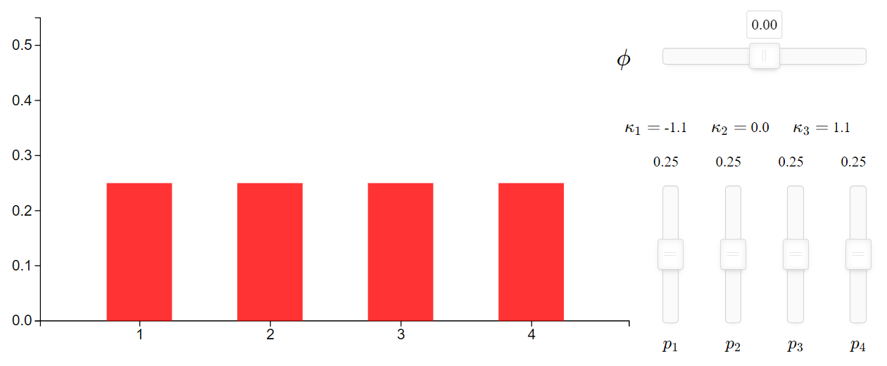
To disentangle these intertwined influences on the final distribution, I’ve built an interactive visualization¹ to help. As shown in the figure above, there are two places where users can tweak to see how the shape of the rating distribution gets influenced.

1. The four vertical sliders are there to adjust the baseline probabilities of the ratings, $Pr(R=1)$, $Pr(R=2)$, $Pr(R=3)$, and $Pr(R=4)$ (abbreviated as $P_1$ ~ $P_4$ respectively). The numerical value on top of each bar indicates the probability of that rating. Note that it is the relative positions between the vertical sliders that matter, and the four probabilities automatically adjust to always sum to one.

   The three values, $\kappa_1$, $\kappa_2$, and $\kappa_3$, shown on top of the four probabilities are the cumulative logits, which are basically the vector of the cumulative probabilities, transformed to the logit scale. They are the baseline latent scores mentioned previously. The last term, $\kappa_4$ is dropped since it is always infinite.

2. The horizontal slider above the vertical sliders controls the value of $\phi$, which gets subtracted from each of the baseline latent scores to derive the final distribution.

Where’s the Regression?

The previous section demonstrates how the baseline rating distribution shifts according to an aggregated influence of $\phi$, which is the hard part of the statistical machinery behind the rating scale IRT model. Regression is the easy part. Now we have a nice and neat $\phi$ sitting on the real space² to work with. If we zoom in on $\phi$, it’s simply the summed effect of the predictor variables in a linear regression, which is similar to $\mu$ in logistic regressions. The only difference here is that we need a different linking distribution to map the effect onto the response scale (i.e., discrete ratings). In math terms, resuming our wine rating example, the distribution is shown in (3):

$$ \begin{aligned} R_i & \sim \text{OrderedLogit}(\phi_i, ~ \bm{\kappa} = \begin{bmatrix} \kappa_1 \\ \kappa_2 \\ \kappa_3 \end{bmatrix} ) \\ \phi_i & = W_{Wid[i]} + J_{Jid[i]} \\ \tag{3} \end{aligned} $$

The $\text{OrderedLogit}$ expression hides all the details from the reader. But you’ve already seen the details at work in code form in previous sections, albeit in a quite scattered manner. Later, I will collect them into a single function. If you prefer clarity now, the monstrous expressions in (4) should suffice.

$$ \newcommand{\logit}{\textrm{logit}} \begin{aligned} R_i \sim \text{Categorical} & ( \begin{bmatrix} \Pr(R_i = 1) = \Pr(R_i \le 1) \phantom{- \Pr(R_i \le 1)} \\ \Pr(R_i = 2) = \Pr(R_i \le 2) - \Pr(R_i \le 1) \\ \Pr(R_i = 3) = \Pr(R_i \le 3) - \Pr(R_i \le 2) \\ \Pr(R_i = 4) = \Pr(R_i \le 4) - \Pr(R_i \le 3) \\ \end{bmatrix} ) \\ \logit[ \Pr(R_i \le 1) ] &= \logit[ Pr(R_i = 1) ] = \kappa_1 - \phi_i \\ \logit[ \Pr(R_i \le 2) ] &= \kappa_2 - \phi_i \\ \logit[ \Pr(R_i \le 3) ] &= \kappa_3 - \phi_i \\ \logit[ \Pr(R_i \le 4) ] &= \logit(1) = \infty \\ \phi_i &= W_{Wid[i]} + J_{Jid[i]} \tag{4} \end{aligned} $$

Don’t worry if you cannot understand the equations in (4) right now. After you get accustomed to the logic of the ordered logit, through coding, the expressions become straightforward. So now let’s wrap up what we have done so far, in code. I will write down the code form of the $OrderedLogit$ distribution in the function rOrdLogit().

 1rOrdLogit = function(phi, kappa) {
 2  kappa = c( kappa, Inf )  # baseline latent scores
 3  L = kappa - phi          # latent scores, after shifting
 4  Pc = logistic(L)         # map latent scores to cumulative probs
 5  # Compute probs for each rating from Pc
 6  Ps = c( 0, Pc )
 7  P = Ps[-1] - Ps[-length(Ps)]  # probs of each rating
 8  sample( 1:length(P), size=1, prob=P )
 9}
10
11## Replicate previous example ##
12P = c( 1, 3, 3, 1 )
13P = P / sum(P)
14Pc = cumsum(P)
15( kappa = logit( Pc )[-length(Pc)] )  # Set up baseline latent scores
16
17# 10,000 draws from OrdLogit
18draws = replicate( 1e4, rOrdLogit(phi=0, kappa=kappa) )  
19# should approach P = c(.125, .375, .375, .125)
20table(draws) / length(draws)

[1] -1.94591  0.00000  1.94591
draws
     1      2      3      4 
0.1282 0.3788 0.3678 0.1252 

Simulating and Fitting Wine Ratings

Having all concepts in place, let’s start synthesizing data for our later model fitting. We will simulate data from the Ordered Logit distribution. One minor limitation with rOrdLogit() defined previously is that it can only take a single value phi, but it is more desirable for phi to be a vector of values. A vectorized version of rOrdLogit() is available in the stom package as rordlogit(). We will be using this function for our data simulation.

 1library(stom)
 2
 3set.seed(1025)
 4Nj = 12  # number of judges
 5Nw = 30  # number of wines
 6J = rnorm(Nj)  # judge leniency
 7W = rnorm(Nw)  # wine quality
 8J = standardize(J)  # scale to mean = 0, sd = 1
 9W = standardize(W)  # scale to mean = 0, sd = 1
10kappa = c( -1.7, 0, 1.7 )  # baseline latent scores
11
12# Create long-form data
13d = expand.grid( Jid=1:Nj, Wid=1:Nw, KEEP.OUT.ATTRS=F )
14d$J = J[d$Jid]
15d$W = W[d$Wid]
16d$phi = sapply( 1:nrow(d), function(i) d$J[i] + d$W[i] )
17d$R = rordlogit( d$phi, kappa )  # simulated rating responses
18d$B = rbern( logistic(d$phi) )   # simulated binary responses
19d$C = rnorm( nrow(d), d$phi )    # simulated continuous responses
20
21# Conversion of data types to match model-fitting function's requirements
22for ( v in c("Jid", "Wid") )
23  d[[v]] = factor(d[[v]])
24d$R = ordered(d$R)
25str(d)

'data.frame':   360 obs. of  8 variables:
 $ Jid: Factor w/ 12 levels "1","2","3","4",..: 1 2 3 4 5 6 7 8 9 10 ...
 $ Wid: Factor w/ 30 levels "1","2","3","4",..: 1 1 1 1 1 1 1 1 1 1 ...
 $ J  : num  0.0187 -0.1794 -1.4372 1.3915 -0.1134 ...
 $ W  : num  0.236 0.236 0.236 0.236 0.236 ...
 $ phi: num  0.2544 0.0564 -1.2014 1.6273 0.1223 ...
 $ R  : Ord.factor w/ 4 levels "1"<"2"<"3"<"4": 4 2 2 2 1 1 1 4 2 3 ...
 $ B  : int  1 0 0 1 1 1 1 1 0 0 ...
 $ C  : num  0.6142 -1.5915 -0.2754 1.2755 0.0792 ...

Running the above code will get our data prepared. Two things might be worth noting. The first is the standardize() function, which centers the input vector to zero mean and a standard deviation of one. J and W are centered here to make the parameters later estimated by the model comparable to the scale of the true values. In our later model, we will partial-pool both the judges and the wines and hence assume a zero-meaned distribution for both of them. Since the sample size of our data isn’t large (12 judges and 30 wines), which will likely cause the means of the raw J and W to have non-minor deviations from zero, standardization is needed.

Second, in addition to R, the rating responses, I also simulate binary responses B (0/1) from phi. Indeed, if a model is fitted with B as the dependent variable, it will be identical to the logistic regression models fitted in previous posts. The binary responses are simulated to demonstrate the parallels between the binary³ model and the rating scale model. The two models are highly similar: the linear effects are aggregated in the same ways (in $\mu$/$\phi$). The only difference is how these effects are projected onto the response scale: the binary model does so through the Bernoulli distribution, and the rating scale model through the Ordered Logit distribution.

Another reason for simulating binary responses along the rating responses is for the preparation of model debugging. As we start fitting more and more complex models, we are bound to find ourselves lost in situations where we have no idea why the model fails to give the expected results. In such cases, it helps a lot to check the results from simpler models, which might hint at where the complex model went wrong. This is also the reason why I simulate the continuous responses C—to prepare data for fitting an even simpler model. By eliminating the influences arising from nonlinear links in the GLMs, the normal response model becomes more transparent and hence much easier to debug.

For our wine rating example here, I’ve deliberately made the data-generating process simple enough that our rating scale model can smoothly fit and give us the expected results. To fit ordered logit regressions with partial pooling structures, we need the clmm() function from the package ordinal. The model syntax in clmm() is basically identical to the syntax we used in lme4::glmer() back then. As shown in the code below, we model the rating scores (R) to be influenced by both the wines and the judges. By partial pooling wines and judges, the wine effects and the judge effects are respectively assumed to come from a zero-meaned normal distribution.

1library(ordinal)
2m = clmm( R ~ (1|Jid) + (1|Wid), data = d )
3summary(m)

Cumulative Link Mixed Model fitted with the Laplace approximation

formula: R ~ (1 | Jid) + (1 | Wid)
data:    d

 link  threshold nobs logLik  AIC    niter    max.grad cond.H 
 logit flexible  360  -455.07 920.14 182(726) 6.96e-06 4.9e+01

Random effects:
 Groups Name        Variance Std.Dev.
 Wid    (Intercept) 1.220    1.1046  
 Jid    (Intercept) 0.853    0.9236  
Number of groups:  Wid 30,  Jid 12 

No Coefficients

Threshold coefficients:
    Estimate Std. Error z value
1|2 -1.42044    0.36491  -3.893
2|3  0.05442    0.35608   0.153
3|4  1.56532    0.36674   4.268

summary(m) prints out the model summary along with the estimated baseline latent scores, which are labeled as Threshold coefficients above. You can see that these coefficients (-1.42, 0.054, and 1.565) align pretty well with the kappa set in the simulation (-1.7, 0, and 1.7).

To examine the estimated wine and judge effects, we similarly utilize the ranef() function as demonstrated in the previous post:

1est_wine = ranef(m)$Wid[[1]]
2est_judge = ranef(m)$Jid[[1]]
3plot( est_wine, W ); abline( 0, 1 )
4plot( est_judge, J ); abline( 0, 1 )

Item Response Theory and Beyond

We have come a long way, from the simplest binary item response model to models with delicate machinery such as the rating scale model with partial-pooling structures. The posts in this demystifying series are sufficient, I suppose, in providing a solid understanding of and practical skills for working with item response theory. There are certainly even more complex IRT models, but I won’t go further in that direction. No matter how many new and complex models are added to the toolkit, we are certain to find our tools in shortage when facing real-world problems.

Item response models, general as they might seem, quickly run out of supply. Although binary and rating scale models allow us to deal with most response types found in the field (such as tests in educational settings, scales measuring psychological constructs, and various surveys used in the social sciences), even the slightest complication renders these models useless. Just consider a mixed-format test consisting of, for example, multiple-choice items (binary scored) and items of open-ended questions (rated). Which IRT model can we apply to this mixed-format test? Not a single one. Instead, we need two separate models, each independently running on a subset of the test for a particular item format. A special technique is then required to map the independently estimated person/item parameters onto a common scale.

The method works but is a waste of information. When models are separately estimated, information cannot be shared across different item formats to improve parameter estimation. Item estimates might be fine, as long as there are many subjects. Person estimates suffer greatly though since, in practice, the test length is limited and is now further divided up by two independent models. This is equivalent to estimating person parameters with fewer items.

It is always better to incorporate everything into a single comprehensive model instead of separately modeling a subset of variables in multiple small models. It is better because information flows smoothly across the variables in a comprehensive model, but the flow breaks down when the model gets torn apart into several pieces. However, such comprehensive models are rarely, if not never, available in the literature. We have to tailor a model ourselves according to what the current situation demands. Therefore, a framework is required to guide us through building up such a model.

This post marks the end of the demystifying series. When the thick cloud of mystery begins to dissolve, we finally get to start solving real and exciting problems rather than wrangling with mad statistical models. In my next post, I will move on to Bayesian statistics, a unified framework that allows flexibly extending a model to match the demanded conditions. Bayesian framework is ideal for empirical research because it is practical. We do not need to wait for a statistician to come up with a model for every new situation. In Bayesian inference, we simply describe the data-generating process and the priors, and the rest is handled by probability theory and an estimation algorithm. Therefore, we can focus on the scientific problems at hand instead of fussing around with fancy models and their names. We will see how item response models can be embedded into a larger network of causes and effects that represents the assumed interactions underlying the current problem. Item response models, which are essentially methods for handling measurement errors, help deal with the latent constructs measured indirectly through surveys in this network of interacting variables.